Company valuation connects financial performance with an investment, acquisition or sale decision. A defensible answer to “What is my company worth?” requires more than multiplying last year’s profit by a sector multiple. It requires a defined valuation date, a clear ownership interest, reliable accounts and assumptions that a buyer can examine.

This guide explains the principal business valuation methods, how their calculations work and how the results inform M&A negotiations. Lev Partners uses discounted cash flow, trading comparables, precedent transactions and adjusted net asset value in its valuation work, selecting and reconciling methods according to the business and assignment.

All companies, forecasts, rates and multiples in the examples are illustrative. They are not client results, current market benchmarks or an offer to buy or sell a business. Unless stated otherwise, amounts are USD millions. Rounded figures may differ slightly.

Start with the right question: enterprise value or equity value?

Enterprise value represents the value of operating activities available to the providers of capital. Equity value represents the residual value attributable to shareholders after relevant financing and other claims. A headline enterprise value is therefore not the cash a seller receives at completion.

The simplified bridge is enterprise value minus financial debt and agreed debt-like items, plus excess cash and separately valued non-operating assets. Minority interests, preferred securities and other claims may require additional adjustments. Normal working capital is generally assumed to be delivered with the operating business; a shortfall or surplus against the contractual target may change the price.

Before modelling, define whether the assignment concerns 100% of the company or a minority holding, a going concern or liquidation, and a market-participant perspective or the value to a particular buyer. Transfer restrictions, voting rights and preferences can make two holdings in the same company worth different amounts per share. Value, asking price and negotiated price are related, but distinct.

1. Discounted cash flow: value the cash the business can generate

A DCF estimates the present value of future cash flows. It is particularly useful when operating drivers can be forecast with reasonable support: production capacity, utilisation, customer retention, contracted sales, pricing, margins, capital expenditure and working capital. A detailed spreadsheet cannot compensate for an unsupported commercial forecast.

Build a forecast from operating drivers

For a manufacturer, revenue can be modelled as units sold multiplied by net selling price, separately for domestic and export business. Gross margin should reflect product mix, raw materials, labour and energy. Receivable days, inventory days and payable days translate growth into working capital needs. Maintenance investment must be distinguished from investment required for new capacity.

Consider an illustrative exporter with revenue of 50.0 and normalised EBITDA of 7.5. In forecast year one, EBITDA is 8.0, depreciation 2.0, tax on operating profit 1.5, capital expenditure 2.0 and the increase in operating working capital 0.5. EBIT is 6.0; after-tax operating profit is 4.5. Free cash flow to the firm is therefore 4.5 + 2.0 − 2.0 − 0.5 = 4.0. The 25% tax assumption is purely illustrative.

EBITDA of 8.0 does not mean 8.0 is distributable. For the five-year valuation case, assume this business produces annual FCFF of 4.0, 4.8, 5.6, 6.3 and 7.0. The first year follows the cash conversion calculation above; subsequent years reflect an illustrative operating forecast, not guaranteed growth.

Match the cash flow to the discount rate

FCFF is discounted at the weighted average cost of capital, or WACC. Free cash flow to equity, after debt cash flows, is discounted at the cost of equity and directly produces equity value. Mixing FCFF with the cost of equity or deducting debt again from an FCFE result produces an inconsistent answer.

WACC combines the cost of equity and after-tax cost of debt using an appropriate capital structure. The cost of equity reflects the currency’s risk-free rate, systematic business risk and relevant risk adjustments. Debt costs should reflect borrowing conditions, not simply the historic coupon. Country and company risks must be considered consistently, without charging for the same risk in several places.

A USD forecast needs a USD-consistent discount rate. A nominal forecast including inflation needs a nominal rate. Converting local-currency revenue into dollars does not remove exchange-rate exposure or country risk. For a group operating in multiple markets, forecast currencies, translation assumptions and intercompany eliminations must reconcile.

What is terminal value, in plain language?

A five-year forecast does not mean the company stops operating after year five. Terminal value summarises the value, at the end of the explicit forecast period, of the cash expected from year six onward. It is not the value of the company today, an extra cash balance, or a guaranteed amount a buyer will pay in five years.

Imagine buying an established manufacturer. You expect to receive value from the first five years of operations, but also from the factory’s continuing business thereafter. A DCF captures the first part year by year and the second part through terminal value. That terminal amount must then be discounted back to the valuation date, just like the earlier cash flows.

In a perpetual-growth model, terminal value equals next year’s normalised free cash flow divided by the discount rate less sustainable growth. Growth must be below the discount rate. The terminal cash flow must include the maintenance investment and working capital required to keep operating and growing. It cannot assume perpetual growth with no associated funding requirement.

If a business has finite concessions, a depleting resource, an expiring contract with no credible renewal or a planned shutdown, perpetual operation may be inappropriate. Model its remaining economic life and any realisable residual assets instead. For an immature company, extend the explicit forecast until the business can reasonably reach a stable state rather than forcing a mature terminal assumption into year five.

A complete five-year DCF calculation

Assume year-end cash flows, WACC of 14% and perpetual growth of 3%. The present value of the five explicit cash flows is 18.35. Year-six normalised FCFF is 7.0 × 1.03 = 7.21. Terminal value at the end of year five is 7.21 ÷ (14% − 3%) = 65.55. Discounting that amount back five years gives 34.04. Enterprise value is consequently 18.35 + 34.04 = 52.39.

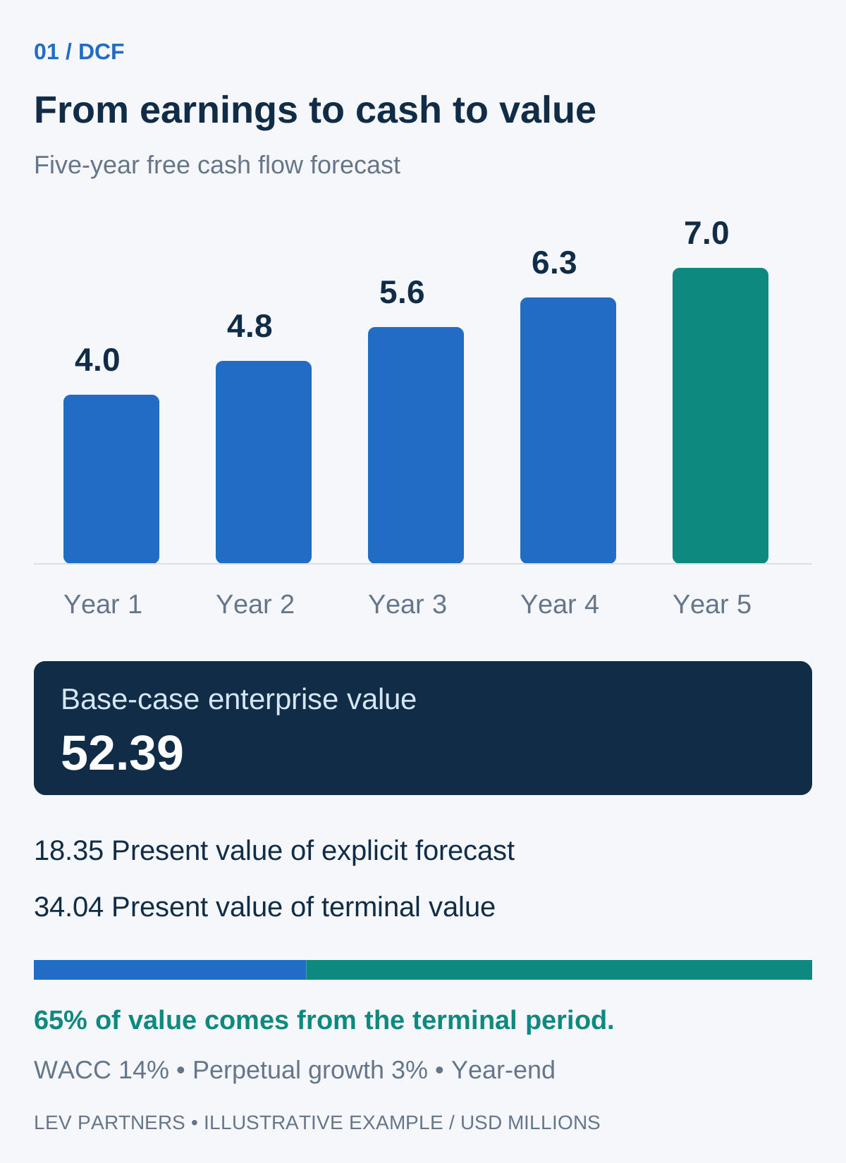
The terminal period contributes approximately 65% of this result. That is a reason to scrutinise assumptions, not a reason to accept the answer automatically. Stable growth must be supported by the reinvestment needed to sustain it. Terminal margins, taxes and capital efficiency should describe a mature business rather than perpetuate an unusually strong year.

An exit-multiple terminal value is another implementation, but it introduces market-pricing assumptions into the DCF. It should be cross-checked against the implied growth and cash conversion. A model should not use both a perpetual-growth terminal value and an exit-multiple value as additive components.

Sensitivity is part of the conclusion

Keeping cash flows unchanged, a 12% WACC and 3% growth produce enterprise value of 64.82. At 16% WACC and 3% growth, the result falls to 43.82. Across the illustrated 12–16% WACC and 2–4% growth matrix, values range from 41.70 to 71.00. This is a sensitivity range, not a statistical confidence interval or a promised sale price.

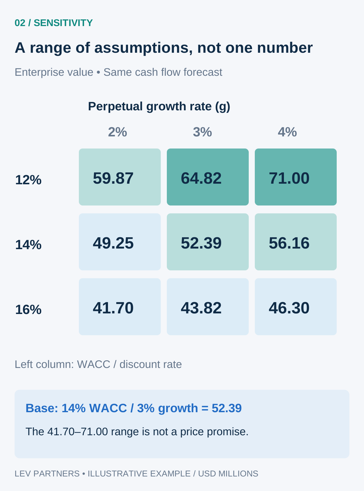
Operating downside cases should also test delayed customer wins, lower utilisation, margin pressure and slower collections. If a project only creates value at the most favourable discount rate and terminal growth combination, the commercial case needs further work.

2. Trading comparables: what does the public market pay for similar businesses?

Trading comparables apply valuation multiples observed for listed peers to a consistently defined financial metric. The work starts with peer selection: business model, geography, scale, growth, margins, customer concentration, cyclicality and capital intensity matter more than a broad industry label.

EV/EBITDA is useful for comparing operating businesses before financing differences, but does not capture capital expenditure. EV/EBIT incorporates depreciation and can help where asset consumption matters. EV/revenue may support analysis of low-profit growth companies, but requires a credible path to sustainable margins. P/E applies to equity earnings and produces equity value, not enterprise value. Price/book needs interpretation alongside returns on equity and asset quality.

For the exporter with normalised EBITDA of 7.5, assume an illustrative selected EV/EBITDA range of 6.0×–8.0×. Enterprise value is 45.0–60.0. These multiples are calculation assumptions, not a claim about what exporters trade at today. An actual engagement would document sources, observation dates, peer exclusions and the reason for the selected range.

Historical and forward multiples must not be mixed. Lease accounting, exceptional expenses and acquisition effects need consistent treatment between the target and peers. A listed company’s scale or liquidity does not justify an arbitrary fixed discount for a private company; any adjustment requires evidence appropriate to the interest being valued.

3. Precedent transactions: learn from completed acquisitions

Transaction comparables examine prices paid for similar businesses. They can reflect control, competitive bidding and buyer-specific synergies, making them relevant to M&A. Their limitation is incomplete disclosure: a reported headline price may exclude assumed debt, earn-outs, retained stakes or working capital adjustments.

Assume comparable completed acquisitions support an illustrative 7.0×–9.0× EV/EBITDA range. Applying it to 7.5 of EBITDA gives enterprise value of 52.5–67.5. Before relying on that range, reconcile each transaction’s enterprise value and financial period, the proportion acquired, contingent consideration and market conditions at signing.

A strategic buyer’s ability to eliminate duplicate costs can explain a premium that another buyer cannot afford. Control is not a universal percentage added to every valuation. If selected transaction multiples already reflect control or synergies, adding a second blanket premium can double count the same benefit.

4. Adjusted net asset value: rebuild the balance sheet economically

Adjusted net asset value values assets and liabilities on an appropriate basis rather than simply accepting book amounts. It is useful for asset-rich businesses, holding companies and situations where earnings do not adequately describe underlying assets. Book equity alone can omit valuable property, obsolete equipment, impaired receivables or liabilities requiring adjustment.

For the same illustrative exporter, suppose adjusted asset values are property 28, machinery 14, inventory 8, receivables 9 and cash 5: total 64. Deduct trade payables of 6, financial debt of 15 and other obligations of 2. Adjusted net asset value is 41, an equity-value result. Adding back debt and debt-like obligations and subtracting excess cash produces an enterprise-value-equivalent bridge of 41 + 15 + 2 − 5 = 53 for comparison with the other methods.

This simplified example assumes the same scope of liabilities and a consistent going-concern basis. Real work may require specialist asset appraisals, tax adjustments, environmental obligations and disposal costs. A profitable operating business can be worth more than its asset base because of customer relationships and organisational capability; an underperforming one may be worth less than an untested replacement-cost total.

Liquidation and replacement cost answer different questions

Liquidation value considers recoverable proceeds after selling costs, claims and the time required to realise assets. An orderly sale and a forced sale have different assumptions. For example, realisations of 38 less obligations of 23 and disposal costs of 3 leave 12 for equity; that is not comparable to a going-concern result without explaining the premise.

Replacement cost estimates the cost of equivalent service capacity, adjusted for physical deterioration and functional or economic obsolescence. It is not simply historic construction cost indexed for inflation. Asset methods should not add operating property to a DCF if the DCF already assumes the business owns and uses that property without rent.

5. Other methods for different business models

Sum of the parts for diversified groups

A group with manufacturing, software and property operations may need separate valuations. If manufacturing enterprise value is 30, software enterprise value 25 and non-operating property value 8, subtract central net debt of 10 and the present value of unallocated corporate costs of 3 to obtain equity value of 50. Eliminate intercompany balances and avoid deducting divisional debt twice. Any holding-company discount must be justified rather than automatically applied.

Dividend and residual income models

A dividend discount model is useful when distributions reasonably represent sustainable shareholder cash flows. An expected next-year dividend of 2, cost of equity of 12% and sustainable growth of 3% imply equity value of 2 ÷ (12% − 3%) = 22.22. A low dividend caused by temporary policy does not necessarily mean low business value.

Residual income starts with book equity and adds the present value of returns above the equity capital charge. With opening equity of 20, net income of 3 and a 12% equity cost, first-year residual income is 3 − 20 × 12% = 0.6. If, purely for illustration, that residual income remains 0.6 indefinitely, value is 20 + 0.6 ÷ 12% = 25. Accounting quality and consistency between earnings and changes in equity are essential.

Early-stage businesses: venture capital and scenario methods

Where near-term cash flows are negative, valuation needs explicit milestones, funding needs, dilution and survival assumptions. Under a simplified venture capital method, an equity exit value of 60 in five years discounted at a 35% target annual return gives present post-money value of approximately 13.38. A new investment of 4 implies pre-money value of 9.38 and approximately 29.9% ownership, assuming no intervening dilution or preference effects.

A probability-weighted scenario model can separately represent failure, moderate growth and successful scale-up. Probabilities must sum to 100%, and terminal proceeds, future funding and timing must be explicit. Do not heavily probability-adjust for failure and then blindly use a discount rate already designed to compensate for the same failure risk. Preferred share rights can require a separate allocation of value among share classes.

LBO analysis and real options

An LBO model tests what a financial sponsor could pay while achieving a target return under a specified debt and cash-generation plan. If exit enterprise value is 80, remaining debt is 20 and the five-year target equity return is 20%, maximum initial equity before other adjustments is 60 ÷ 1.2⁵ = 24.11. With initial debt financing of 25, that suggests an enterprise purchase capacity of 49.11, ignoring fees, interim distributions and other claims. Debt must be supportable; this is a buyer-return constraint, not a universal fair value.

Real-option analysis can help value a genuine right to defer, expand or abandon a project. The right must be identifiable and economically meaningful. An expansion opportunity is not automatically an extra asset added on top of a DCF that already includes the expansion cash flows.

From valuation to M&A: what actually changes the cheque?

Return to the DCF enterprise value of 52.39. Deduct financial debt of 15 and debt-like items of 2, then add excess cash of 5. Equity value is 40.39, assuming normal working capital is delivered and no other adjustments. A 1.2 working-capital shortfall against the agreed target would reduce that to 39.19 if the contract provides a dollar-for-dollar adjustment.

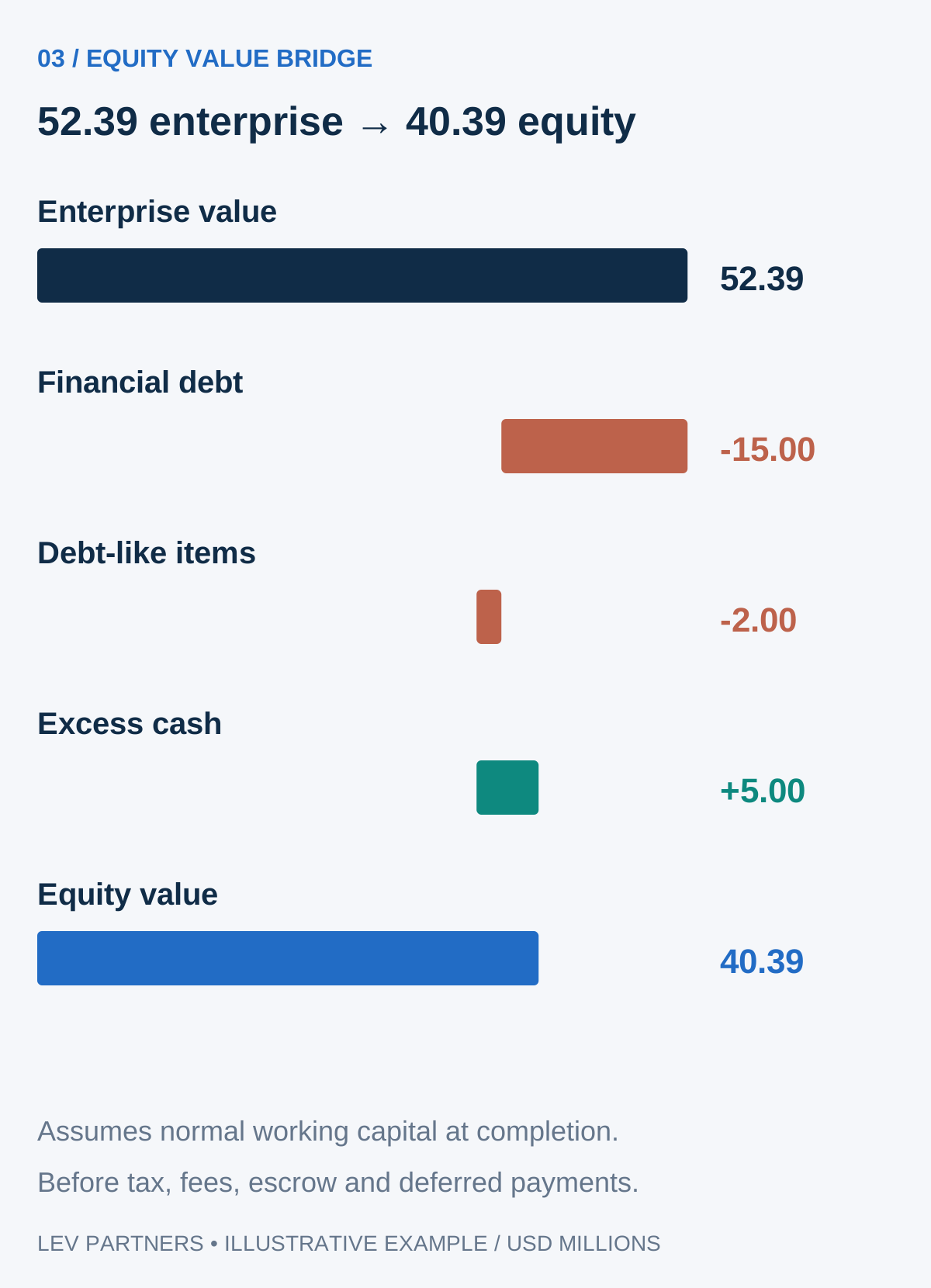
Cash at completion can be lower again because of escrow, deferred consideration, fees and taxes. Compare an offer of 40 in cash with one of 44 comprising 32 at completion and a conditional earn-out of 12: the larger headline is not automatically better. Timing, performance conditions, buyer credit and the seller’s ability to influence future results matter.

Financial due diligence tests normalised earnings and debt-like exposures. Adding back an owner’s exceptional expense is only defensible if it will genuinely disappear and any replacement cost is recognised. A customer loss after the valuation date, overdue receivables or an unfunded capacity requirement can affect both the valuation and contractual protections.

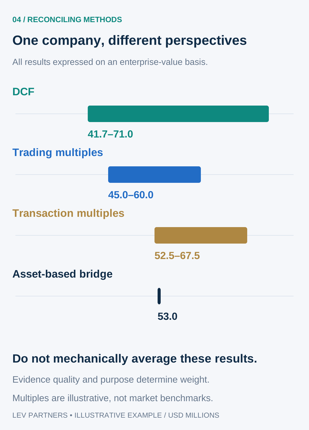
Reconciliation is a reasoned judgement, not the average of four spreadsheets. A reliable DCF may carry greater weight for a business with visible cash flows; weak forecasts may shift attention to market evidence. Asset values can provide a separate perspective, but are not an automatic floor. Explain why a method receives more or less weight and present the conclusion on a consistent enterprise or equity basis.

The Lev approach: understand earnings quality before applying a multiple

At Lev Partners, valuation begins with the economic nature of the business. We examine quality of earnings (QoE), the quality of cash conversion and the underlying records rather than treating reported EBITDA as a ready-made valuation input. The aim is to identify sustainable operating earnings, the investment required to produce them and the risks that affect their realisation.

From the general ledger to the commercial explanation

Within the agreed scope and available access, our review moves from financial statements into ledger entries, invoices, credit notes, customer and supplier balances, bank movements and transaction-level samples. We connect accounting entries to delivery, billing, collection and payment. Revenue cut-off, returns after year-end, related-party transactions, capitalised operating costs and exceptional income can change the earnings base. Transaction-level review is not a claim that every transaction is audited or that a financial-statement audit opinion is provided.

Consider reported EBITDA of 8.0. A non-recurring legal cost of 0.4 may be added back, but a non-recurring operating grant of 0.6 may need to be removed. If replacing an underpaid owner-manager costs another 0.3 annually, normalised EBITDA becomes 8.0 + 0.4 − 0.6 − 0.3 = 7.5. Each adjustment needs evidence. At an illustrative 7× multiple, using unadjusted EBITDA would overstate enterprise value by 3.5. An add-back is not valid simply because management labels an expense “one-off”.

Cash-flow quality depends on the sector’s operating cycle

We analyse receivable and payable terms against the business model, customer contracts, seasonality and relevant sector evidence. A 90-day collection period can mean something different for an OEM supplier with accepted contractual terms than for a consumer business that normally collects immediately. A longer contractual term is still a funding requirement; being normal for the sector does not make it costless or risk-free.

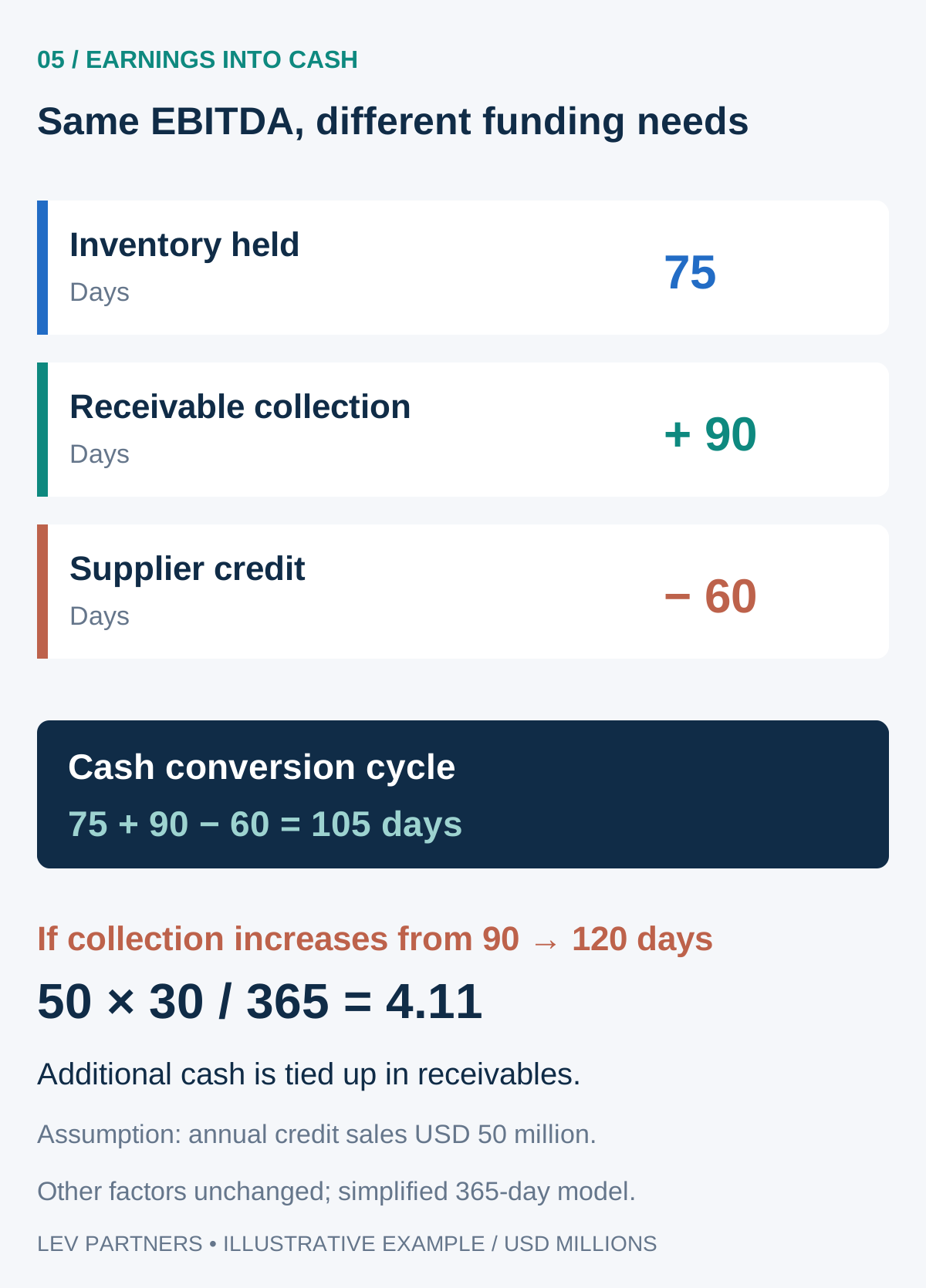
Suppose annual credit sales are 50 and annual cost of goods sold is 35, with 90 receivable days, 75 inventory days and 60 payable days. Using a simplified 365-day model, receivables are 12.33, inventory 7.19 and payables 5.75. Operating working capital is approximately 13.77, and the cash conversion cycle is 90 + 75 − 60 = 105 days. Actual analysis should use average or monthly balances and appropriate purchase denominators where needed.

If receivable days rise to 120 while everything else remains unchanged, an additional 50 × 30 ÷ 365 = 4.11 is tied up in receivables. EBITDA can look unchanged even as financing needs increase. That is why we examine ageing, subsequent receipts, disputes, concentration, factoring and whether suppliers are being paid late. Cash released by stretching suppliers beyond agreed terms is not necessarily sustainable operating improvement.

Sector, country and brand change the valuation logic

For an industrial company we may focus on maintenance capex, utilisation and customer programmes; for software, recurring revenue, churn and acquisition costs; for branded consumer products, price premiums, repeat purchases, channel margins and the spending required to sustain demand. The same revenue or EBITDA multiple cannot be transferred between these businesses without testing the economics.

Country analysis considers cash-flow currency, customer geography, inflation, funding conditions, transfer restrictions where relevant and the enforceability and stability of contracts. We distinguish the company’s registered location from the markets where it earns and collects money. Risks reflected in forecast scenarios must be reconciled with discount-rate adjustments to avoid double counting.

Brand can support value through demonstrable pricing power, customer retention or licensing income. Where the assignment requires a separate intangible-asset analysis, a relief-from-royalty approach estimates the present value of after-tax royalties that owning the brand avoids, using supportable licensing assumptions and a defensible economic life. For example, 20 of branded revenue at an illustrative 2% royalty and 25% tax gives a first-year after-tax royalty saving of 0.30, before further required modelling. That is a cash-flow input, not a complete brand valuation.

If the operating DCF already captures the brand’s higher prices and margins, adding a separately calculated brand value on top can count the same benefit twice. Our objective is a coherent company valuation informed by its distinctive economics, not a collection of premiums attached to the same business.

How Lev Partners connects valuation with execution

Our valuation work uses DCF, trading comparables, precedent transactions and adjusted net asset value, as appropriate. We connect the analysis to the client’s decision: preparing a company sale, considering an acquisition, negotiating an investment or evaluating ownership alternatives. U.S.-based, with a presence in Turkey, Lev Partners supports clients across international markets.

1. Define scope: valuation date, entities, shareholding, purpose and basis of value.

2. Establish the financial baseline: reconcile accounts, normalise earnings and identify debt, cash and working-capital items.

3. Build and challenge projections: connect sales drivers, margins, capex and funding requirements.

4. Apply and reconcile methods: document assumptions, peer selection and sensitivity ranges.

5. Translate value into transaction terms: support positioning, buyer discussions, due diligence, negotiation and completion mechanics within the agreed mandate.

Useful starting documents include three years of financial statements, current management accounts, debt and cash schedules, working-capital ageing, fixed-asset records, the budget, customer concentration and the ownership structure. Better information can reduce uncertainty; it does not guarantee a particular multiple or a completed transaction.

Frequently asked questions about company valuation

Can a company be valued using revenue alone?

A revenue multiple is a cross-check in appropriate sectors, not a substitute for analysing margins, retention, cash conversion and funding needs. Two companies with the same sales can have very different values.

Is EBITDA multiplied by a sector number enough?

No. The earnings base must be normalised, the selected multiple supported and the enterprise-to-equity adjustments reconciled. Forward and historical figures need consistent treatment.

Does a 30% stake equal 30% of the full-company equity value?

That is a starting arithmetic allocation, not always the final answer. Voting rights, transfer restrictions, liquidation preferences and the purpose of the valuation can change the value of the specific interest.

How long does a valuation take?

Timing depends on data quality, group complexity, the purpose and specialist work required. The scope and deliverables should be agreed after an initial information review rather than promised before the business is understood.

Discuss your valuation and transaction options

Erim N. Kargacı — Founding Partner and Head of M&A

Erim leads Lev Partners’ M&A advisory, supporting company owners in investment, acquisition and company sale processes.

Explore our M&A advisory services, or contact us today to discuss your company’s valuation, the information needed and the transaction alternatives relevant to your objectives.

Further reading

International Valuation Standards Council: valuation standards; Aswath Damodaran, NYU Stern: Investment Valuation resources; CFA Institute: Free Cash Flow Valuation; CFA Institute: Residual Income Valuation. Examples and illustrations in this article were prepared for educational purposes by Lev Partners.